This project draws on two complementary data sources to investigate whether gold functions as an inflation hedge through the lens of physical trade flows. UN Comtrade data captures what flows where between countries, while the World Bank Global Inflation Database captures the inflationary environment the country was in at the time. Joining the two on country and year lets us test whether the trade patterns of gold (and its peers silver and platinum) respond to inflation in the way the popular narrative suggests.
All raw inputs live under data/raw/. Reproducible build scripts in data/build_dataset.py and data/country_mapping.py generate the processed outputs in data/processed/. The original Kaggle UN Comtrade dump ends in 2016, which was a problem for our 2022–23 inflation-wave question — so we added a second, more recent UN Comtrade extract (1990–2025) midway through the project to extend the coverage.
1 Raw data
1.1 Overview Raw Datasets
Table 1: Overview of raw datasets used in the project.
Name
Source
Storage location
Size
UN Comtrade — Global Commodity Trade Statistics (1988–2016)
Kaggle dataset by Uciml, derived from UN Comtrade
data/raw/commodity_trade_statistics_data.csv
~1.2 GB
UN Comtrade — Precious Metals (1990–2025)
UN Comtrade Database (HS chapter 71 extract, codes 7106–7112)
data/raw/comtrade_1990_2025.csv
~24 MB
World Bank Global Inflation Database
Ha, Kose & Ohnsorge (2023), One-Stop Source: A Global Database of Inflation, World Bank
data/raw/Inflation-data.xlsx
~5.6 MB
1.2 Details Dataset 1
Content. Country-level commodity trade statistics from the United Nations Comtrade database, redistributed on Kaggle. Covers virtually every traded commodity (HS classification) for 1988–2016, with import / export / re-import / re-export flows, USD values, weights and physical quantities.
Source / provider. Kaggle dataset “Global Commodity Trade Statistics” by user uciml, derived from the UN Comtrade Database (https://comtradeplus.un.org). UN Comtrade itself is maintained by the United Nations Statistics Division.
Procurement. Downloaded once from Kaggle via the kagglehub Python package. The file is large (~1.2 GB) and not committed to git; team members re-acquire it with:
Legal aspects. The Kaggle redistribution is published under the Creative Commons CC0 1.0 (public domain) license. The underlying UN Comtrade data is subject to the UN Statistics Division terms of use (free non-commercial use with attribution).
Data governance. Public, non-personal, business-relevant aggregate trade statistics. No sensitive or personal data.
Role in the analysis. Provides the dependent / target family of variables in our narrative: trade value in USD and weight in kilograms of precious-metals flows.
1.2.1 Data Catalogue
Table 2: Data catalogue for the UN Comtrade legacy dataset (raw columns kept after filtering to HS 7106–7112).
#
Column name
Datatype
Values / validation
Description
1
country_or_area
string
263 country / area names, free-text
Reporting country
2
year
int
1988 – 2016
Calendar year of the trade flow
3
comm_code
string
HS 6-digit code, here filtered to 7106–7112
Harmonized System commodity code
4
commodity
string
Free-text commodity description
Human-readable commodity name
5
flow
category
Import, Export, Re-Import, Re-Export
Direction of the trade flow
6
trade_usd
int
≥ 0, USD
Trade value in current US dollars
7
weight_kg
float
≥ 0, kg (some missing)
Net weight
8
quantity_name
string
e.g. Weight in kilograms, Number of items
Unit of quantity
9
quantity
float
≥ 0
Physical quantity in the unit above
10
category
string
HS chapter group, e.g. 71_pearls_precious_stones_metals
Aggregated commodity category
1.2.2 Data Characteristics and Quality
The full file has ~8.2 M rows across all commodities. After filtering on commodity descriptions containing “Gold”, “Silver”, “Platinum” or “precious metal” in build_dataset.py, we retain ~190 k rows on HS chapter 71 metals — well above the 500-row course minimum and the right order of magnitude for country–year aggregates.
Findings from EDA:
Coverage. 263 reporting countries or areas, every year from 1988 to 2016. Coverage is densest from the mid-1990s onward — most early-1990s post-Soviet states only start reporting in 1995–1996.
Missing values. Weight is missing in roughly 11 % of precious-metals rows (small jewellery items reported only as a count). Trade value in USD is never missing.
Zero values. About 9 % of rows have a zero weight, almost all for fabricated articles (rings, coins) where the reporting country dropped weight reporting.
Skew. Trade value is strongly right-skewed (median ≈ 73 k USD, max ≈ 97 bn USD — a 2014 Switzerland gold import row). A log scale will be required for any scatter visualization.
Negative values. None — the raw data is sign-clean.
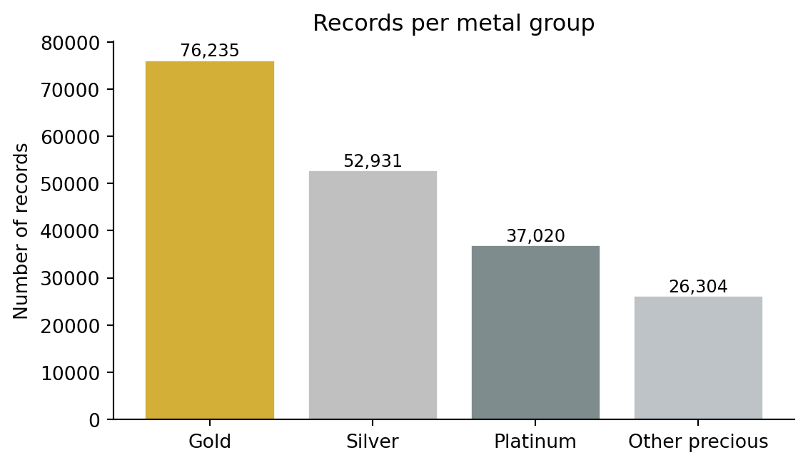
Commodity cardinality. Around 25 distinct precious-metals commodity strings. We collapse these into four metal groups (Gold, Silver, Platinum, Other precious) in processing.
Flow imbalance. Imports dominate the rows (~82 %), reflecting the fact that more countries report imports than exports for HS 71.
Code
import pandas as pdimport matplotlib.pyplot as plttrade = pd.read_csv("../data/processed/precious_metals_trade_1988_2024.csv")counts = trade["metal_group"].value_counts().reindex( ["Gold", "Silver", "Platinum", "Other precious"])fig, ax = plt.subplots(figsize=(6, 3.5))bars = ax.bar(counts.index, counts.values, color=["#D4AF37", "#C0C0C0", "#7F8C8D", "#BDC3C7"], edgecolor="white")ax.set_ylabel("Number of records")ax.set_title("Records per metal group")for s in ("top", "right"): ax.spines[s].set_visible(False)for bar, val inzip(bars, counts.values): ax.text(bar.get_x() + bar.get_width() /2, bar.get_height(),f"{val:,}", ha="center", va="bottom", fontsize=9)plt.tight_layout()plt.show()
Figure 1: Number of precious-metals trade records by metal group in the processed dataset (1988–2024).
Implications for visualisation. The heavy right-skew in trade values forces a log scale on any “value vs. inflation” scatter (Chapter 2 of the story). The 11 % missing weights mean we will lead with trade value for cross-country comparisons and use weight only as a secondary lens for top reporters where it is dense.
1.3 Details Dataset 2
Content. A focused extract from the official UN Comtrade Plus API for HS codes 7106–7112 (silver, gold, platinum, semi-manufactured forms, waste & scrap, coins), covering 1990 to 2025.
Procurement. Pulled directly through the UN Comtrade REST API and saved as a single CSV. We added this dataset after discovering that the Kaggle dump ended in 2016, which made it impossible to study the 2022–23 inflation spike directly. The newer extract is much narrower than the Kaggle dump (only HS 71 codes, only the BACI / Comtrade harmonized fields) but extends coverage by nine extra years.
Legal aspects. UN Comtrade is free for non-commercial use with attribution. Bulk redistribution is permitted under the same terms.
Data governance. Public, non-personal.
Role in the analysis. Same target variables as Dataset 1 (primary trade value and net weight), used to extend the time series past 2016.
1.3.1 Data Catalogue
The full extract has 46 columns; the ones we retain are listed below. Columns dropped early include estimation flags, customs codes and mode-of-transport metadata that are not relevant for country–year aggregates.
Table 3: Retained columns from the UN Comtrade 1990–2025 extract.
#
Column name
Datatype
Values / validation
Description
1
refYear
int
1990 – 2025
Reference year
2
reporterISO
string
ISO-3 code, e.g. AUS
Reporting country code
3
reporterDesc
string
Country name
Reporting country, free-text
4
flowCode
category
M, X, RM, RX
Import / Export / Re-Import / Re-Export
5
partnerISO
string
ISO-3 code or W00 (World)
Trade partner code
6
cmdCode
string
HS codes 7106 – 7112
HS commodity code
7
cmdDesc
string
HS description
Free-text commodity description
8
netWgt
float
≥ 0, kg, may be empty
Net weight
9
primaryValue
float
≥ 0, USD
Primary trade value (CIF for imports, FOB for exports)
10
qty
float
≥ 0
Reported physical quantity
1.3.2 Data Characteristics and Quality
71,843 rows for HS 7106–7112 globally. ISO codes are clean (no manual fuzzy matching needed). The 2017–2025 portion is the main reason this dataset exists — earlier years overlap with Dataset 1 but use slightly different harmonisation revisions, so we do not stack the two raw files: Dataset 1 provides 1988–2016 and Dataset 2 provides 2017–2024 in the merged output.
1.4 Details Dataset 3
Content. Country-level inflation rates by indicator (Headline CPI, Food CPI, Energy CPI, Core CPI, PPI, GDP deflator), at monthly, quarterly and annual frequency. We use only the annual sheets for joining with annual trade data.
Procurement. Manually downloaded once from the World Bank brief page as Inflation-data.xlsx and committed to data/raw/. The file is small enough (~5.6 MB) that we keep it in the repo for easy reproducibility.
Legal aspects. World Bank data is released under the Creative Commons CC-BY 4.0 license. Attribution to Ha, Kose & Ohnsorge (2023) is required and given in the references.
Data governance. Public, non-personal, official macroeconomic statistics.
Role in the analysis. Provides the independent / regressor variables: country-year inflation rates. We use Headline CPI as the primary driver and Food / Energy / Core CPI as secondary lenses to answer research question 5 (“Which type of inflation has the strongest link to gold trade activity?”).
1.4.1 Data Catalogue
The Excel workbook contains 20 sheets. Each annual sheet (hcpi_a, fcpi_a, ecpi_a, ccpi_a, ppi_a, def_a) is one wide table with year columns 1970–2024.
Table 4: Structure of one annual inflation sheet (e.g. hcpi_a).
#
Column name
Datatype
Values / validation
Description
1
Country Code
string
ISO-3 alpha code
World Bank ISO-3 code
2
IMF Country Code
int
Numeric IMF country identifier
IMF country code
3
Country
string
205 country / aggregate names
Country name in World Bank spelling
4
Indicator Type
string
Inflation
Constant within a sheet — useful when sheets stacked
5
Series Name
string
e.g. Headline Consumer Price Inflation
Series description
6 – 60
1970 … 2024
float
Inflation rate in % year-on-year, may be blank
One column per year
61
Note
string
e.g. Annual average inflation
Methodology note
1.4.2 Data Characteristics and Quality
Coverage. 205 countries, 4 CPI types used (Headline / Food / Energy / Core), 55 years (1970–2024). After melting to long format the indicator dataset has roughly 50,000 rows with non-missing inflation values.
Missing values. Coverage is shallowest before 1990 and for low-income countries — e.g. Food and Energy CPI series only begin in the 1990s for many emerging economies.
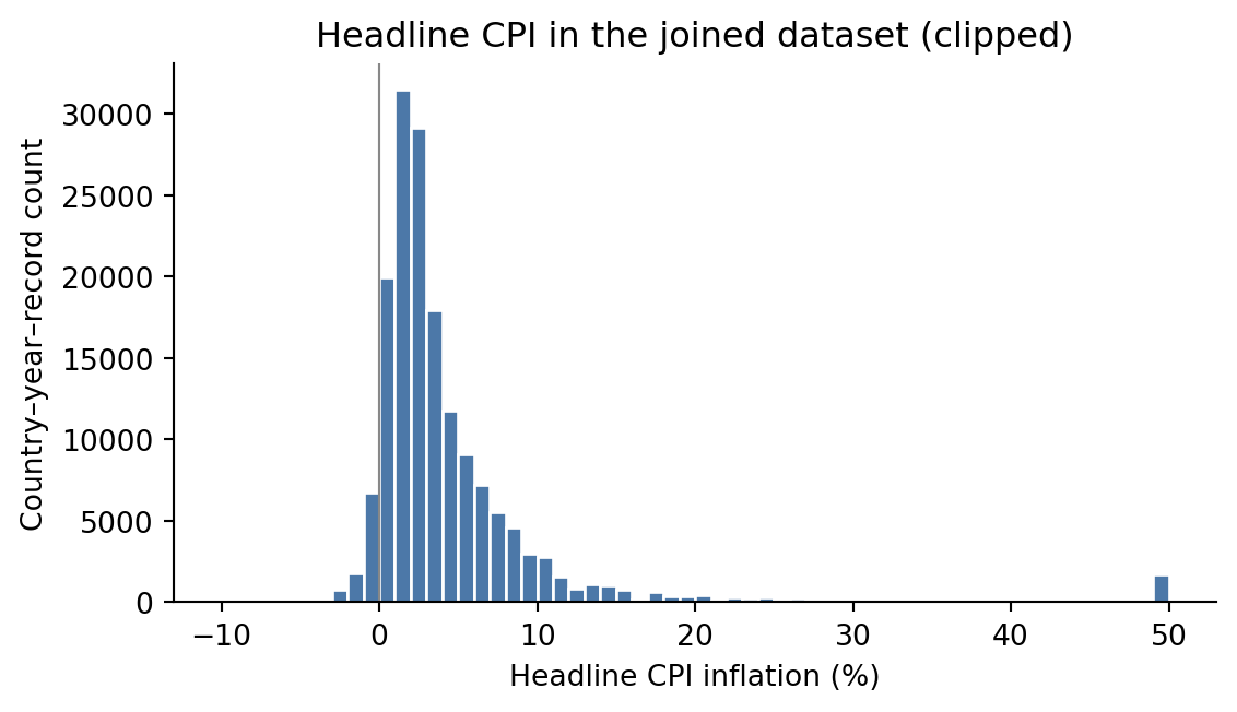
Extreme values. Inflation has very long tails: minimum –73 % (deflationary spikes), maximum 65,374 % (Venezuela 2018 hyperinflation). For visualisation we will clip or use a symlog axis; for statistical summaries we use medians.
Country naming. World Bank uses names like “Egypt, Arab Rep.” while UN Comtrade uses “Egypt”. This is the main reason country_mapping.py and the in-script COUNTRY_MAP dictionary exist.
Code
import pandas as pdimport matplotlib.pyplot as plttrade = pd.read_csv("../data/processed/precious_metals_trade_1988_2024.csv")cpi = trade["Headline CPI"].dropna().clip(-10, 50)fig, ax = plt.subplots(figsize=(6, 3.5))ax.hist(cpi, bins=60, color="#4C78A8", edgecolor="white")ax.axvline(0, color="#888", linewidth=0.8)ax.set_xlabel("Headline CPI inflation (%)")ax.set_ylabel("Country–year–record count")ax.set_title("Headline CPI in the joined dataset (clipped)")for s in ("top", "right"): ax.spines[s].set_visible(False)plt.tight_layout()plt.show()
Figure 2: Distribution of annual Headline CPI inflation in the merged dataset, clipped to [-10, 50] % for readability. Values beyond the clip points (Zimbabwe, Venezuela, etc.) are real but flatten the histogram if left in.
Implications for visualisation. The fat right tail justifies symmetric-log or clipped axes in the scatter plot of Chapter 2. The shallow pre-1990 coverage means most chart defaults should start at 1995 to keep the global panel balanced.
2 Processed Data
2.1 Overview Processed Datasets
Table 5: Overview of processed datasets produced by data/build_dataset.py and data/country_mapping.py.
Table 7: Per-column missing / zero rates and basic ranges for the main processed dataset.
n_missing
pct_missing
n_zero
min
max
country
0
0.0
0
NaN
NaN
year
0
0.0
0
1988.000000
2.024000e+03
metal_group
0
0.0
0
NaN
NaN
flow
0
0.0
0
NaN
NaN
trade_value_usd
0
0.0
0
1.000000
9.696865e+10
weight_kg
20479
10.6
16745
0.000000
1.640361e+09
Headline CPI
28750
14.9
58
-72.728996
6.537408e+04
Key takeaways:
No duplicates on the natural key of country, year, metal group and flow — verified during build.
Inflation join rate is 85 % overall; the unmatched 15 % is overwhelmingly micro-states and territories (e.g. Cook Islands, Falkland Islands) absent from the World Bank database — acceptable for a global story.
Country mismatch residual. After the manual country mapping, ~14 small trade entities still have no inflation partner; they are kept in the dataset with a missing Headline CPI but excluded from inflation-conditional charts at render time.
Outliers. A handful of country-year cells exceed 10 bn USD in gold trade (Switzerland 2011–2014, UK 2010–2014). These are real refining-hub flows, not data errors, and they are central to the Swiss-connection chapter — we keep them and rely on log axes.
Implications. Coverage and quality are sufficient for all five planned chapters. The two design decisions forced by the data are: (i) log axes wherever trade value or inflation appears, and (ii) showing the unmatched country slice as a separate row count rather than letting it silently disappear.
2.3 Details Processed Dataset 2
Content. Country-year gold imports only, drawn from a BACI-style harmonisation of UN Comtrade for 2017–2024, joined with Headline CPI.
Reason it exists. The Chapter 2 scatter plot (inflation vs. gold imports) is most compelling for the recent inflation spike. This narrower dataset gives a cleaner, smaller frame for that specific chart without dragging the full 1988–2024 panel into a single scatter.
Processing. Filter to Gold imports only on the 1990–2025 UN Comtrade extract, then left-join Headline CPI on country and year. Same naming-harmonisation as Dataset 1.
2.3.1 Data Catalogue
Same schema as Dataset 1, but restricted to gold imports. Year range 2017–2024.
2.3.2 Data Characteristics and Quality
50,331 rows over 224 countries. Headline CPI is missing for ~11 % of rows (same micro-state pattern as the main dataset). No further cleaning is applied — this is a view onto the joined data, not a new pipeline.
2.4 Details Processed Dataset 3
Content. Two-column lookup table mapping every country name appearing in the trade data to an ISO-3166 alpha-2 code, used for choropleth rendering in Plotly (which expects ISO codes, not names).
Processing. Generated by data/country_mapping.py using a three-step strategy:
Exact match against the pycountry library by name.
Fuzzy fallback via pycountry’s fuzzy search.
Manual overrides for ~30 known mismatches (“Korea, Rep.” → KR, “Hong Kong SAR, China” → HK, etc.).
Quality. 191 of 263 distinct country strings map to a valid ISO-2 code. The remaining ~70 are sub-national entities, historical aggregates (“Fmr Sudan”, “Neth. Antilles”) or non-country reporters (“Other Asia, nes”, “Bunkers”); they appear in the trade data but are not plottable on a country map and are filtered out of choropleths.